Artificial Intelligence
1 Search
1.1 Agent Design
There are mainly two types of agents.
Reflex Agents: Choose action based on current percept (and maybe memory), may have memory or a model of the world's current state, do not consider the future consequences of their actions.
Planning Agents: Decisions based on (hypothesized) consequences of actions, must have a model of how the world evolves in response to actions, and must formulate a goal (test).
1.2 Search Problems and Algorithms
Search Problems
A state space.
A successor function (with actions, costs).
A start state and a goal test.
A solution is a sequence of actions (a plan) which transforms the start state to a goal state.
State Space Graphs vs. Search Trees
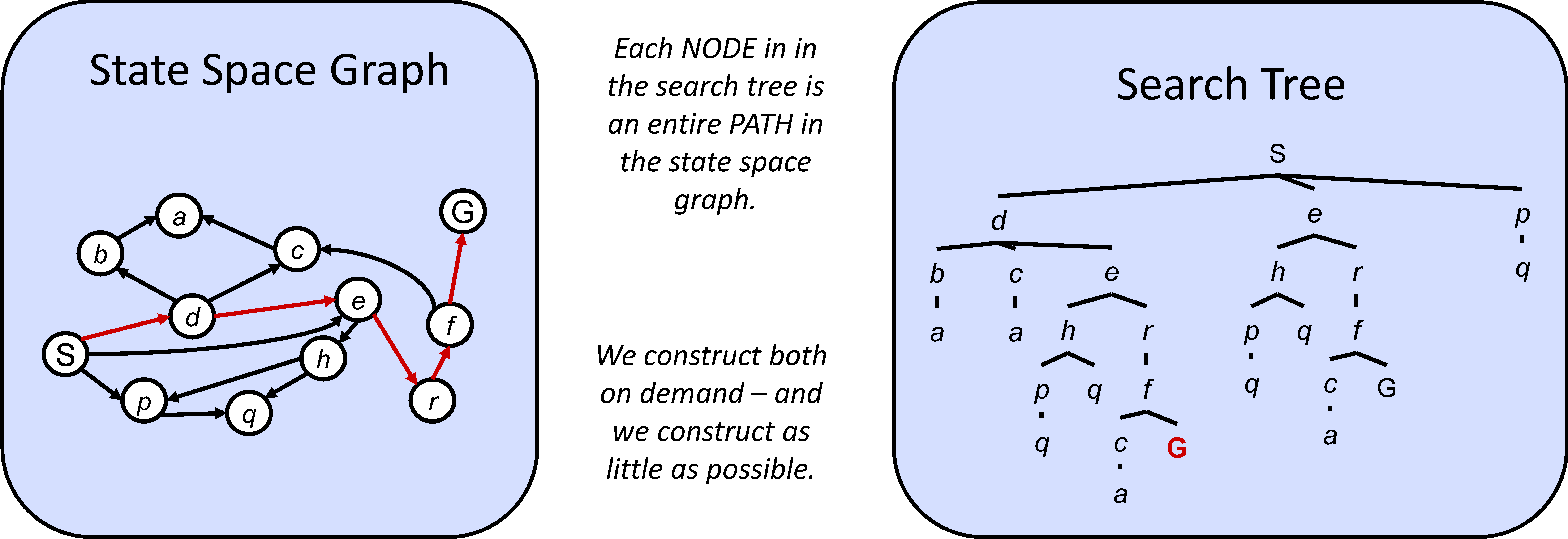
Search Algorithms
Uninformed search algorithms (blind search)
Depth-First Search
Breadth-First Search
Uniform-Cost Search
Informed search algorithms (heuristic search)
A* Search
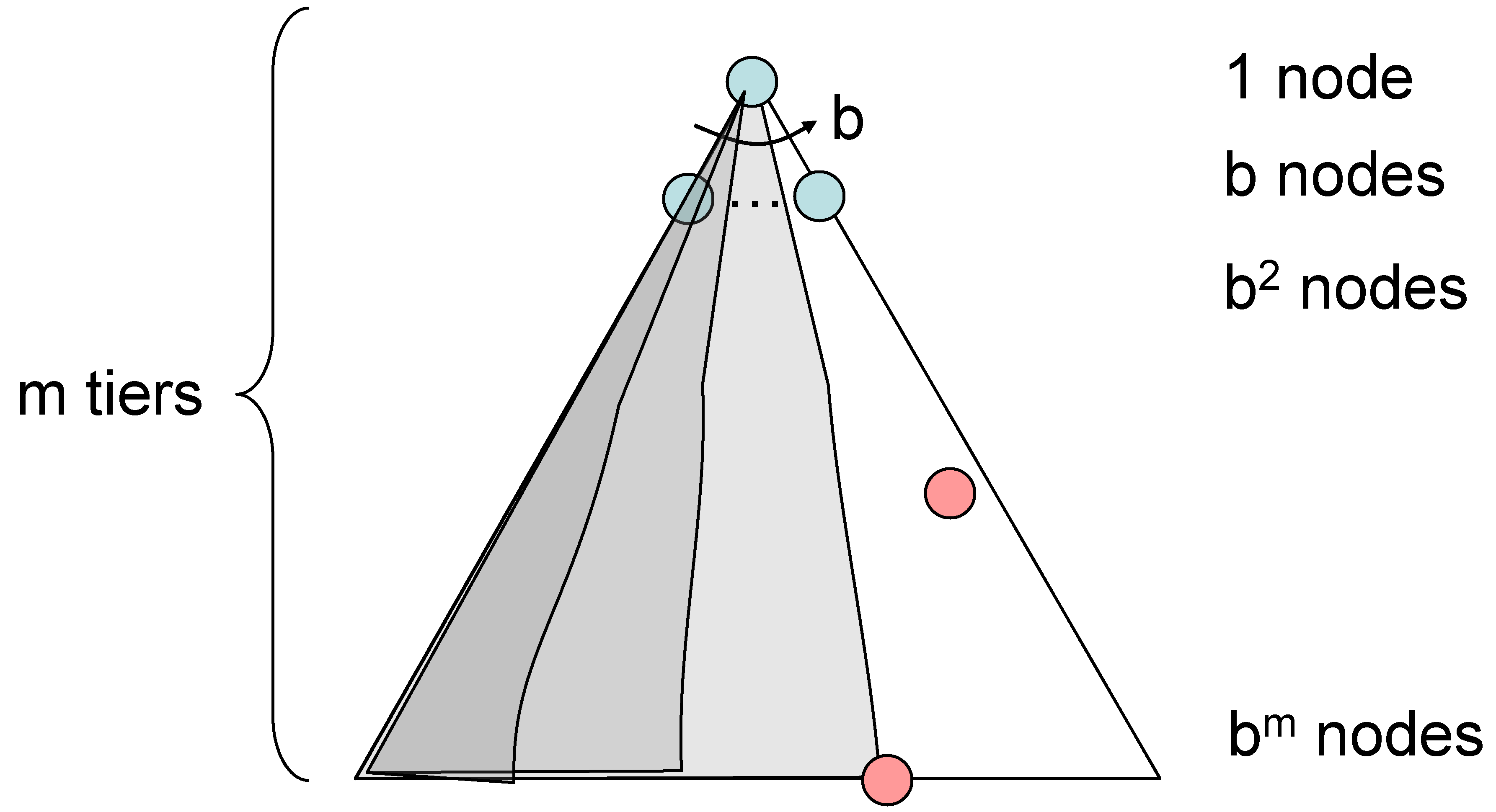
Depth-First Search
Completeness:
could be infinite, so only if we prevent cycles. Optimality: No, it finds the "leftmost" solution, regardless of depth or cost.
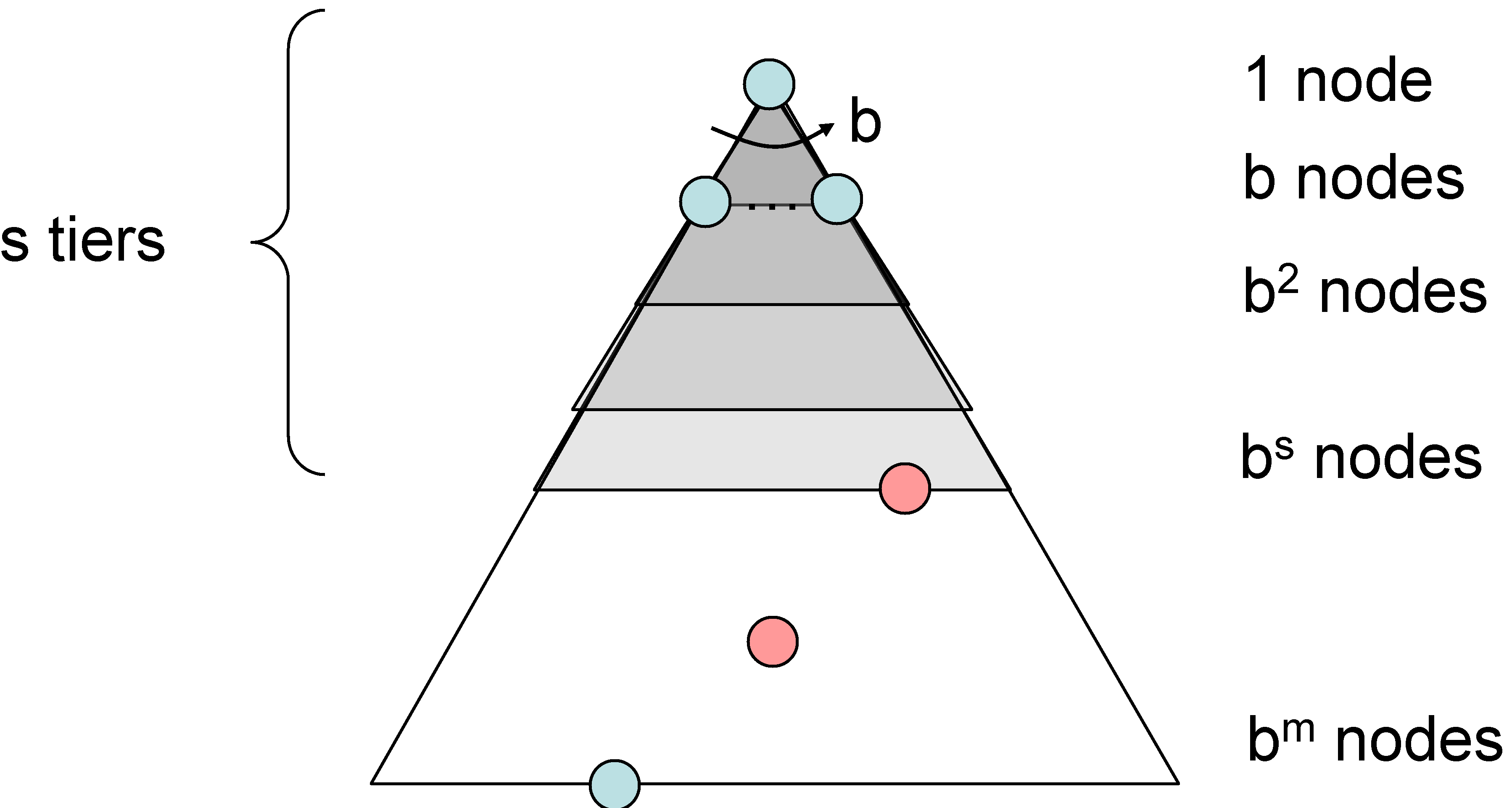
Breadth-First Search
Completeness:
must be finite if a solution exists , so yes! Optimality: Only if costs are all 1.
Iterative Deepening: get DFS’s space advantage with BFS's time / shallow solution advantages, run Run a DFS with depth limit 1, 2, 3, ...
1.2.1 Uniform Cost Search
Uniform Cost Search: Expand the node with the lowest path cost.
Uniform Cost Search
Dequeue the node with the lowest path cost (current_node).
If current_node is the goal state, reconstruct and return the path.
Expand current_node: For each successor (neighbor) of current_node,
If the successor is not in the explored set and not already in the priority queue, create a new node for the successor with the calculated cost and parent set to current_node, and insert the successor node into the priority queue.
Else if the successor is already in the priority queue with a higher cost, update the successor's cost in the priority queue and its parent to current_node.
If that solution costs
and arcs cost at least , then the "effective depth" is roughly . Time complexity:
Space complexity:
Completeness: Assuming best solution has a finite cost and minimum arc cost is positive, yes!
Optimality: Yes!
1.2.2 Heuristics (A* Search)
In AI, A heuristic is a function that estimates how close a state is to a goal in a search problem.
Greedy Search: Strategy: Expand a node that you think is closest to a goal state using heuristic.
Combining UCS & Greedy Search
Uniform cost orders by path cost, or backward cost
. Greedy orders by goal proximity, or forward cost
. A* Search orders by the sum:
.
Admissibility
Inadmissible (pessimistic) heuristics can break optimality by overestimating the cost to reach the goal, so A* may not find the actual optimal path.
Admissible (optimistic) heuristics slow down bad plans but never outweigh true costs.
A heuristic h is admissible (optimistic) if,
where
Optimality of A* Search
Assume
Proof
Imagine
n will be expanded before B
is less or equal to . is less or equal to . expands before .
All ancestors of
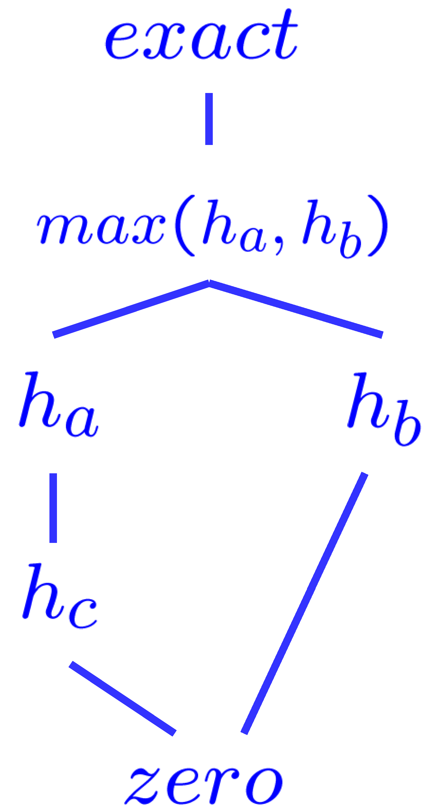
Semi-Lattice of Heuristics
Dominance:
if , Max of admissible heuristics is admissible. By comparing, we want the best heuristic possible , one that's as close to the true cost as you can get while still being admissible.
Top of lattice is the exact heuristic, which would be the exact cost.
2 Constraint Search Problem
Constraint Satisfaction Problems (CSPs): A special subset of search problems, for which states is defined by variables
Binary CSP: Each constraint relates (at most) two variables.
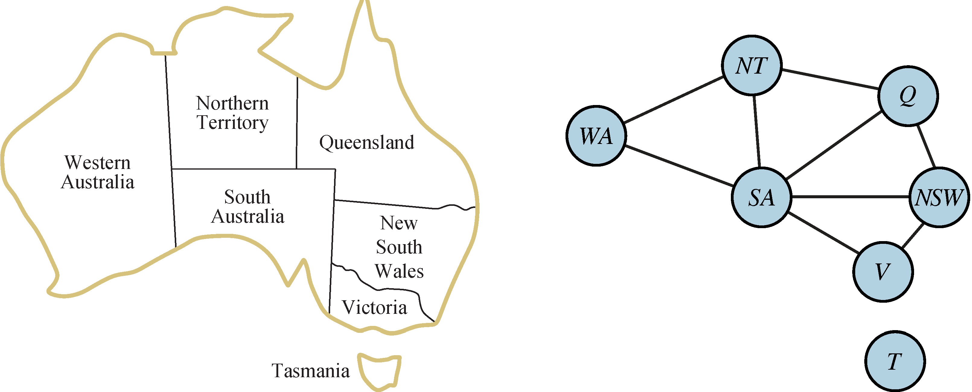
Binary constraint graph: Nodes are variables, arcs show constraints.
Varieties of CSPs
Discrete Variables
Finite domains: Size
means complete assignments, e.g., Map Coloring, N-Queen, Boolean CSPs, including Boolean satisfiability (NP-complete). Infinite domains (integers, strings, etc.): E.g., job scheduling, variables are start/end times for each job; linear constraints solvable, nonlinear undecidable.
Continuous Variables: E.g., start/end times for Hubble Telescope observations, linear constraints solvable in polynomial time by linear programming methods.
Varieties of Constraints
Unary constraints: Involve a single variable (equivalent to reducing domains), e.g.:
. Binary constraints: involve pairs of variables, e.g.:
. Higher-order constraints: Involve 3 or more variables, e.g., cryptarithmetic column constraints.
2.1 Backtracking Search
Backtracking Search: DFS, along with variable ordering (i.e., [WA = red then NT = green] same as [NT = green then WA = red]) and constraints checking as you go (i.e., consider only values which do not conflict with previous assignments).
Filtering
Forward checking propagates information from assigned to unassigned variables, but doesn't provide early detection for all failures.
For example, in the example of mapping colors for Australia above, if WA is red, then NT & SA cannot be red; if we choose Q to be green next, there is a problem: NT & SA cannot all be blue, but we didn't detect this!
Consistency of A Single Arc: An arc X -> Y is consistent iff for every
in the tail there is some in the head which could be assigned without violating a constraint. 
In this example, Arc SA to NSW is consistent: for every x in the tail there is some y in the head which could be assigned without violating a constraint.